In the modern era, most organizations went data-driven, and all of their decisions are curate through data. Every day, a large amount of data gets generated and handled by powerful computers led by artificial intelligence algorithms. Data science and machine learning are driving these enormous data to fetch valuable insights for the betterment of business decisions. In this article, you will learn what linear regression is and how it helps in various data analysis.
What is Linear Regression?
Linear Regression is one of the most prominent and initial data science and machine learning algorithms that every data science professional & machine learning engineer comes across. It is a simple statistical model that everyone should understand because it lays the base-level framework for other ML algorithms. It is popularly used in predictive analysis.
There are two goals of performing linear regression analysis. First, it checks whether the predictor variable is doing a proper job in predicting an outcome (dependent) variable or not, and second, which variables, in particular, are significant predictors of the outcome variable?
When can we use Linear Regression?
Linear regression analysis usually requires some phenomenon of interest and several observations having at least two or more features. Considering the assumption, we can note that (at least) one of the characteristics depends on the others. Data analysts and data scientists can establish a relation among them through this. In other words, we can say that it is a function that maps some features or variables to others adequately.
We can use this powerful method to recognize the circumstances that influence profitability. Forecasting sales for the future month, predicting the customer's requirement, and other future analyses can be done using the data extracted from the existing months and leveraging linear regression with it. Data scientists can also use linear regression to understand various insights related to customer behavior. Linear regression also helps in predicting the weather, temperature, number of residents in a particular house, economy of a country, electricity consumption, etc.
Regression Performance:
The variation of original responses 𝑦ᵢ,𝑖 =1,…,𝑛, happens partially due to the dependency on the predictor variable 𝐱ᵢ. Nevertheless, it also comes with an extra inherent variety of output. The coefficient of determination (𝑅²) indicates the amount of variation in 𝑦 described by the dependence on 𝐱 using the accurate regression model. Larger 𝑅² denotes a better match. It also determines that the model can describe the output's variation with varying inputs.
Types of Linear Regression:
There are two different variations of linear regression. The type mostly depends on the number of independent variables being used in the linear regression function.
Simple Linear Regression:
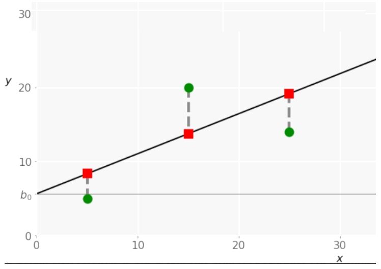
Simple or single-variate linear regression is the most simplistic type of linear regression. The entire regression analysis depends on one independent variable, 𝐱 = 𝑥. When executing simple linear regression, you have to start giving a set of input-output (𝑥-𝑦) marks with pairs. These pairs are the observations, and the distances created between these observations are the optimal values and the predicted weights 𝑏₀ and 𝑏₁ that determine the predicted regression function.
Multiple Linear Regressions:
Multiple linear regressions or a multivariate linear regression is a type of linear regression having two or more independent variables. When it will have only two independent variables, the expected regression function becomes (𝑥₁, 𝑥₂) = 𝑏₀ + 𝑏₁𝑥₁ + 𝑏₂𝑥₂. This equation becomes a regression plane in a 3-dimensional space. Its goal is to define the values of the weights 𝑏₀, 𝑏₁, and 𝑏₂ in a manner that the plane is as close as feasible to the original responses.
Python Program for Linear Regression:
import numpy as np
import matplotlib.pyplot as mpl
def estim_coef(x, y):
    nn = np.size(x)
    m_x = np.mean(x)
    m_y = np.mean(y)
    SS_xy = np.sum(y*x) - nn * m_y * m_x
    SS_xx = np.sum(x*x) - nn * m_x * m_x

    # here we will calculate the regression coefficients
    b_1 = SS_xy / SS_xx
    b_0 = m_y - b_1*m_x

    return (b_0, b_1)

def regression_line(x, y, b):
    mpl.scatter(x, y, color = "y",
               marker = "+", s = 40)

    y_pred = b[0] + b[1]*x
    mpl.plot(x, y_pred, color = "b")
    mpl.xlabel('x')
    mpl.ylabel('y')

    mpl.show()

def main():
    x = np.array([0, 1, 2, 3, 4, 5, 6, 7, 8, 9])
    y = np.array([2, 4, 5, 6, 7, 8, 8, 9, 9, 11])
    b = estim_coef(x, y)
    print("Estimated coefficients:\nb_0 = {}  \
          \nb_1 = {}".format(b[0], b[1]))
    regression_line(x, y, b)

if __name__ == "__main__":
    main()
Output:
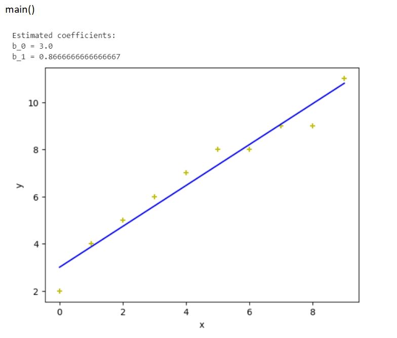
Explanation:
First, we have imported numpy and Matplotlib.pyplot as np and mpl (as their alias name). Next we created a user-defined function name estim_coef() using the def keyword, having two parameters x and y. Within the function, we have created np.size(x) and stored in a variable nn. Similarly, we have calculated the mean of x and stored in m_x and the mean of y in m_y.
Finally we calculated the sum of both of them individually and stored in SS_xy and SS_xx variables. Then, we have calculated the regression coefficients storing the calculated value in b_1 and b_0. Then we returned both of them back to the function.
Next, we created another user-defined function regression_line() having three parameters x, y, and b. This function is meant to plot all the calculations done in the previous program. We used the scatter plot (mpl.scatter()) and set the color, marker symbol, and size. Also, this function body contains the line graph of the x and y_pred and label it as xlabel and ylabel. Also, we have pushed a separate color to the line (blue using the color code b).
Finally we have to define the main() where we have created np.array() and passed the list [0, 1, 2, 3, 4, 5, 6, 7, 8, 9] and stored the entire Numpy array in x. Similarly, we have to create another Numpy array [2, 4, 5, 6, 7, 8, 8, 9, 9, 11] and store it in y. Finally, we print the lines and plots by calling the function regression_line().
Advantages of Linear Regression:
- Linear Regression becomes easy, manageable, and easy to interpret in the form of output coefficients.
- When there is a correlation between the independent and dependent variable having a linear connection, this algorithm can be the most suitable to use because of its less complexity as compared to other regression techniques.
Disadvantages of Linear Regression:
- In the linear regression algorithms, outliers can produce large effects on the regression, where the boundaries are linear.
- The way a mean is not a complete representation of a single variable, the linear regression technique also does not completely describe the relationships among variables.
Conclusion:
Linear regression is one of the most useful tools of statistics used in data science to analyze the relationships among the variables. Although, it is not recommended in all possible applications because this technique over-simplifies real-world problems by considering a linear relationship among the variables within a relation.
But it is the fundamental statistical and machine learning technique and therefore, there is a good chance that you might need to understand its basic requirements.