Data Science is one of the most emerging domains & most sought-after career opportunities. It uses scientific approaches, statistical methods, computer science algorithms, and operations to obtain facts & insights from different forms of datasets. To predict the user requirements, organizational insights, operational cost analysis, and other analytical visualizations, data science is a proven tool.
Among its various approaches, probability distribution plays a vital role in delivering data analysis. This article will guide you with the top categories & types of probability distribution methods, techniques, and Python programs data analysts use for analyzing large datasets.
Probability Distribution in Python:
A Probability Distribution is a function of statistics that helps in describing the likelihood of achieving the potential values from random variables. It determines all the possibilities that a random variable can present from a range of values. This range contains a lower bound and an upper bound that comprise the minimum & the maximum possible values require to analyze from the dataset.
There are multiple circumstances on which different analytics value depends. Among them, standard deviation, average, and skewness are prominent. Probability distribution empowers data analysts to identify and perceive patterns from large data sets. Thus, it plays a crucial role in summarizing which data set to consider from a large cluster of semi-structured and unstructured data. Data science using Python allows density function & distribution techniques to plot data, visually analyze data and extract insights from them.
General Properties of Probability Distributions:
Probability distribution defines the possibility of any consequence from a given data set. This mathematical expression uses a precise value of x and determines the likelihood of a random variable with p(x). Probability distribution follows some general properties listed below –
- The result of all possibilities for any feasible value tends to become equal to 1.
- When a probability distribution method is applied to any data, the possibility of any particular value or a range of values must lie in the range of 0 & 1.
- Probability distributions is meant to show the dispersal of the values. Accordingly, the type of variable helps in determining the standard of probability distribution.
List of some well-known Probability distributions used in Data Science:
Here is a list of the popular types of Probability distribution explained with a python code that every data science aspirant should know. (Use Jupyter Notebook to practice them)
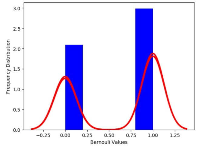
Bernoulli Distribution:
It is one of the simplest and common probability distribution types. It uses the concept of Binomial distribution, where n=1. It means a binomial distribution takes 'n' number of trials, where n > 1 whereas, the Bernoulli distribution takes only a single trial. The Bernoulli Probability distribution will accept n number of trials, known as Bernoulli Trials. Any random experiment will have one of the two outcomes (either a failure or a Success). The Bernoulli event is the action based on which the probability of occurrence of the event is 'p', and the probability of the event not occurring is '1-p'.
Program:
import seaborn as sb
from scipy.stats import bernoulli
def bernoulliDist():
bernoulli_data = bernoulli.rvs(size = 860, p = 0.6)
    aw = sb.distplot(bernoulli_data,  kde = True,  color = 'b', hist_kws = {'alpha' : 1}, kde_kws = {'color': 'r', 'lw': 3, 'label': 'KDE'})
aw.set(xlabel = 'Bernouli Values', ylabel = 'Frequency Distribution')

bernoulliDist()
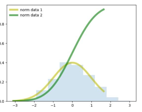
Normal Distribution:
It is also known as Gaussian distribution, which is another popular probability distribution that is symmetric around the mean. It helps in displaying that the data near the mean are more frequent as compared to the occurrences of data far from the mean. In this case, mean = 0, variance = finite value.
Program:
import numpy as np
import matplotlib.pyplot as mpl
from scipy.stats import norm
def normalDistri() -> None:
    fig, aw = mpl.subplots(1, 1)
    mean, vari, skew, kurt = norm.stats(moments = 'mvsk')
    xx = np.linspace(norm.ppf(0.001),  norm.ppf(0.95), 90)
aw.plot(xx, norm.pdf(xx),
        'y-', lw = 5, alpha = 0.6, label = 'norm data 1')
aw.plot(xx, norm.cdf(xx),
        'g-', lw = 5, alpha = 0.6, label = 'norm data 2')
vals = norm.ppf([0.001, 0.5, 0.999])
np.allclose([0.001, 0.5, 0.999], norm.cdf(vals))
    r = norm.rvs(size = 2000)
aw.hist(r, normed = True, histtype = 'stepfilled', alpha = 0.2)
aw.legend(loc = 'best', frameon = False)
mpl.show()

normalDistri()
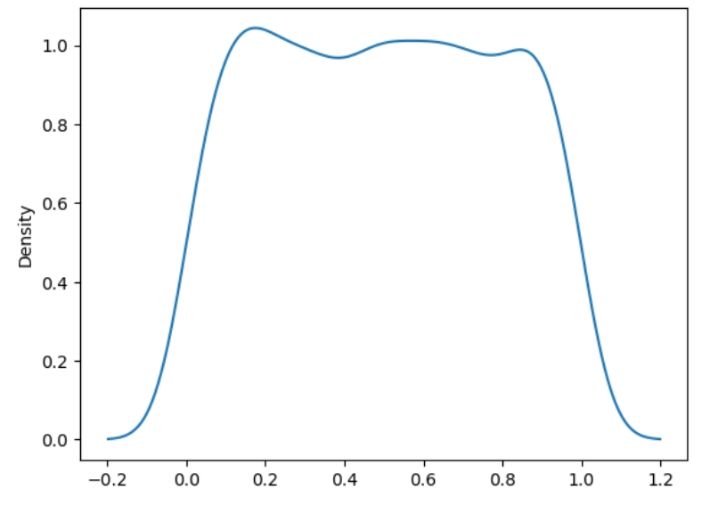
Continuous distribution:
In this type of probability distribution, all the outcomes from a given set of execution are equally possible. All the variable or values residing within the range gets the same hit of possibility as a consequence. Such symmetric probabilistic distribution gets a chance to have a random variable at an even interval, having the probability of 1/(b-a).
Program:
import matplotlib.pyplot as mp
from numpy import random
import seaborn as sbrn
def contDist():
sbrn.distplot(random.uniform(size = 1600), hist = False)
mp.show()

contDist()
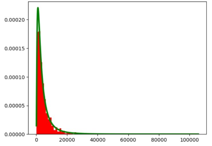
Log-normal distribution:
It is a form of a continuous distribution; the log form of the variable will have a normal distribution. Programmers and statistics professionals can reconstruct the data into normal distribution from a log-normal distribution.
Program:
import numpy as np
import matplotlib.pyplot as mp
def lognormDistri():
mue, sigma = 8, 1
    s = np.random.lognormal(mue, sigma, 1000)
cnt, bins, ignored = mpl.hist(s, 85, normed = True, align ='mid', color = 'r')
    xx = np.linspace(min(bins), max(bins), 10000)
    calc = (np.exp( -(np.log(xx) - mue) **2 / (2 * sigma**2))
           / (xx * sigma * np.sqrt(2 * np.pi)))
mp.plot(xx, calc, linewidth = 3.0, color = 'g')
mp.axis('tight')
mp.show()

lognormDistri()
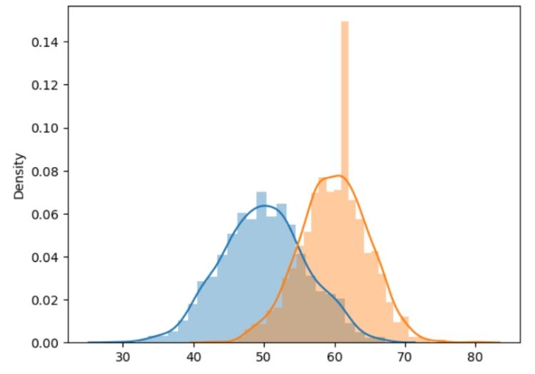
Binomial Distribution:
It is the most well-known distributions technique for separating data that define the likelihood of success 'x' having 'n' trial(s). The binomial distribution is popularly implemented in situations where data analysts want to extract the probability of SUCCESS or FAILURE of any data prediction. Data from an experiment, dataset, or survey has to go through several routines. A Binomial distribution executes a fixed amount of trials. Its events have to be independent & the chance of getting a failure or success must remain the same.
Program:
from numpy import random
import matplotlib.pyplot as mp
import seaborn as sbrn
def binoDist():
sbrn.distplot(random.normal(loc = 50, scale = 6, size = 1400), hist = True, label = 'normal dist')
sbrn.distplot(random.binomial(n = 100, p = 0.6, size = 1400), hist = True, label = 'binomial dist')
mp.show()

binoDist()
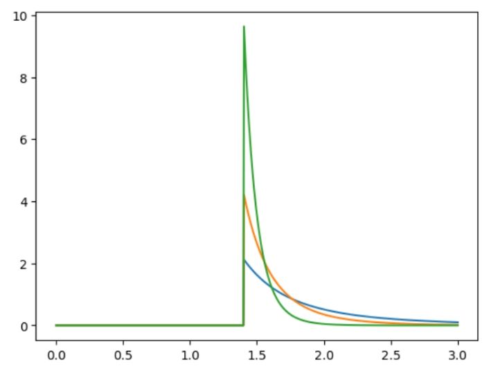
Pareto Distribution:
It is a continuous distribution, defined by a shape parameter, α. It is a skewed statistical distribution that is used for modeling the distribution of incomes and/or city population. It uses power law for describing quality control, social, experimental, actuarial, and different types of observable phenomena. This probability distribution focuses mainly on the larger outcome as compared to the smaller.
Program:
import numpy as np
from matplotlib import pyplot as mp
from scipy.stats import pareto
def paretoDistri():
xm = 1.4
alph = [3, 6, 14]
    xx = np.linspace(0, 3, 700)
    output = np.array([pareto.pdf(xx, scale = xm, b = aa) for aa in alph])
mp.plot(xx, output.T)
mp.show()

paretoDistri()
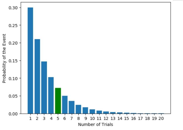
Geometric Distribution:
The geometric probability distribution is one of the special types of negative binomial distributions deals with the count of trials needed for a single success. This probability distribution helps in determining any event that have the likelihood 'p' and that will occur after 'n' Bernoullian trials. Here 'n' is a discrete random variable, and the experiment iterates again and again until it reaches a success or a failure.
Program:
import matplotlib.pyplot as mpl

def probability_to_occur_at(attempt, probability):
    return (1-p)**(attempt - 1) * probability

p = 0.3
attempt = 4
attempts_to_show = range(21)[1:]
print('Possibility that this event will occur on the 7th try: ', probability_to_occur_at(attempt, p))
mpl.xlabel('Number of Trials')
mpl.ylabel('Probability of the Event')
barlist = mpl.bar(attempts_to_show, height=[probability_to_occur_at(x, p) for x in attempts_to_show], tick_label=attempts_to_show)
barlist[attempt].set_color('g')
mpl.show()
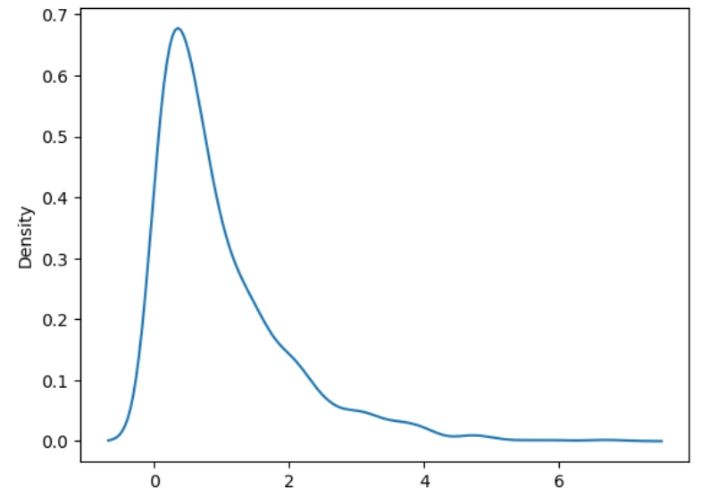
Exponential Distribution:
It is the probability distribution that talks about the time between different events. It determines which process from the event have occurred in a continuous fashion and independently at a constant average rate.This distribution also defines the time elapsed between events (in a Poisson process).
Program:
from numpy import random
import matplotlib.pyplot as mp
import seaborn as sbrn
def expoDistri():
sbrn.distplot(random.exponential(size = 1400), hist = False)
mp.show()

expoDistri()
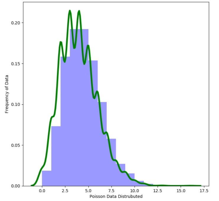
Poisson Distribution:
It is one of the well-accepted forms of discrete distribution that reveals the number of times an event will possibly happen in a particular time frame. We can achieve this by narrowing down the Bernoulli distribution from 0 to any number. Data analysts implement this Poisson distribution to embrace independent events happening at a specific time interval and a constant rate.
Program:
from scipy.stats import poisson
import seaborn as sbrn
import numpy as np
import matplotlib.pyplot as mp

def poissonDistri():
mp.figure(figsize = (8, 8))
data_binom = poisson.rvs(mu = 4, size = 4600)
    ae = sbrn.distplot(data_binom, kde=True, color = 'b',
                    bins=np.arange(data_binom.min(), data_binom.max() + 1.4),
kde_kws={'color': 'g', 'lw': 4, 'label': 'KDE'})
ae.set(xlabel = 'Poisson Data Distrubuted', ylabel='Frequency of Data')
mp.show()

poissonDistri()
Conclusion:
Although each of these distribution techniques has its own significance and use, the most popular of these probability distributions are Binomial, Poisson, Bernoulli, and Normal Distribution. Today, enterprises and firms are hiring data science professionals for different departments, namely, various engineering verticals, insurance sector, healthcare, arts & design, and even social science, where probability distributions act as the core tool for filtering data from a parge dataset and use those data for valuable insight. Therefore, every data science professional and data analyst should know their use.